Please pay attention.)
One important example is a position
![]() and a momentum
and a momentum
![]() of a particle
of a particle ![]() .
.
(Note for physicists: we employ a "system of units" such that the Planck's constant (divided by
Then the expectation of a function
![]() (say) when the state
corresponds to a
(say) when the state
corresponds to a ![]() function
function ![]() is given by
is given by
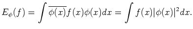
One may then regard
![]() as a ``probability density'' of the
particle
as a ``probability density'' of the
particle ![]() on
on
![]() .
.
![]() is called the wave function of the particle.
We should note:
is called the wave function of the particle.
We should note:
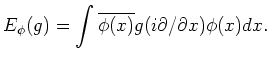
On the other hand,
the expectation of a function
![]() should be:
should be:
The computation becomes easier when we take a Fourier transform ![]() of
of ![]() .
.
= (2 \pi)^{-n/2} \int f(x) e^{i x \xi} d x
$](img78.png)
or its inverse
= (2 \pi)^{-n/2} \int f(x) e^{-i x \xi} d x
(=\mathcal{F}[g](-\xi)).
$](img79.png)
The Fourier transform is known to preserve the ![]() -inner product. That means,
-inner product. That means,
One of the most useful properties of the Fourier transform is that it transforms derivations into multiplication by coordinates. That means,
Using the Fourier transform we compute as follows.
![$\displaystyle E_\phi(g)=
\int \overline{\mathcal{F}[\phi]}g(-\xi) \mathcal{F}[\...
...al{F}[\phi]\vert^2 d x.
=\int g(\xi) \vert\mathcal{\bar{F}}(\phi) \vert^2 d x.
$](img82.png)
We then realize that
![]() plays the role of the probability density
in this case.
plays the role of the probability density
in this case.
Thus we come to conclude:
The probability amplitude of the momentum is the Fourier transform of the probability amplitude of the position.
The Fourier transform, then, is a way to know the behavior of quantum phenomena.
| One may regard a table of Fourier transform (which appears for example in a text book of mathematics) as a vivid example of position and momentum amplitudes of a particle. |
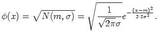
To illustrate the idea, let us know concentrate on the case where ![]() and assume that
and assume that ![]() is a square root of the
normal(=Gaussian) distribution
is a square root of the
normal(=Gaussian) distribution
![]() of mean value
of mean value ![]() and standard deviation
and standard deviation ![]() .
.
By using a formula
![$\displaystyle \mathcal{F}[e^{-x^2/a}]=\sqrt{\frac{a}{2}}e^{-a \xi^2/4},
$](img90.png)
we see that the Fourier transform of
![$\displaystyle \mathcal{F}[\phi]=\sqrt{\frac{1}{\sqrt{2 \pi}\sigma^{-1}/\sqrt{2}...
... (\sigma^{-1}/\sqrt{2})^2} }
=e^{i \xi m}\sqrt{N(0,\frac{1}{\sqrt{2}\sigma})},
$](img91.png)
so that the inverse Fourier transform is given as follows.
![$\displaystyle \bar{\mathcal{F}}[\phi]
=e^{-i \xi m}\sqrt{N(0,\frac{1}{\sqrt{2}\sigma})}.
$](img92.png)
We observe that
both ![]() and
and
![]() are normal distribution,
and that the standard deviation of them are inverse proportional to each other.
are normal distribution,
and that the standard deviation of them are inverse proportional to each other.
In easier terms, the narrower the ![]() distributes,
the wider the transform
distributes,
the wider the transform
![]() does.
does.
It is a primitive form of the fact known as ``the uncertainty principle''.